Using R to Understand Benchmarking Results
Why R?
Evaluating benchmark results with Excel became too cumbersome and error prone for me so that I needed an alternative. Especially, reevaluating new data for the same experiments was a hassle. However, the biggest problem with Excel was that I did not know a good way to query the raw data sets and group results easily to be able to answer different kind of questions about the data. Thus, I decided I need to learn how to do it in a better way. Since, I was not really happy with the debuggability, traceability, and reusability of my spreadsheets either, I gave up on Excel entirely. I bet, Excel can do most of the things I need, but I wanted a text-based solution for which I can use my normal tools, too.
While working on ReBench, I got already in touch with matplotlib to generate simple graphs from benchmark results automatically. But well, Python does not feel like the ultimate language for what I was looking for either. Instead, R was mentioned from time to time when it came to statistical evaluation of measurements. And, at least for me, it turned out to be an interesting language with an enormous amount of libraries. Actually, a bit to enormous for my little needs, but it looked like a good starting point to brush up on my statistics knowledge.
By now, I use it regularly and applied it to a number of problems, including my work on the RoarVM and a paper about CSOM/PL.
Benchmark Execution
Before we can analyze any benchmark results, we need a reliable way to execute them, ideally, as reproducible as possible. For that purpose, I use a couple of tools:
- ReBench
- A Python application that executes benchmarks based on a given configuration file that defines the variables to be varied, the executables to be used and the benchmarks and their parameters.
- SMark
- A Smalltalk benchmarking framework that allows one to write benchmarks in a style similar to how unit-tests are written.
- Codespeed
- This is mostly for the bigger picture, a web application that provides the basic functionality to track long-term performance of an application.
Beside having good tools, serious benchmarking requires some background knowledge. Today’s computer systems are just to complex to get good results with the most naive approaches. In that regard, I highly suggest to read the following two papers which discussing many of the pitfalls that one encounters when working with modern virtual machines, but also just on any modern operating system and with state-of-the-art processor tricks.
- Georges, A.; Buytaert, D. & Eeckhout, L. Statistically Rigorous Java Performance Evaluation SIGPLAN Not., ACM, 2007, 42, 57-76. (PDF)
- Blackburn, S. M.; McKinley, K. S.; Garner, R.; Hoffmann, C.; Khan, A. M.; Bentzur, R.; Diwan, A.; Feinberg, D.; Frampton, D.; Guyer, S. Z.; Hirzel, M.; Hosking, A.; Jump, M.; Lee, H.; Moss, J. E. B.; Phansalkar, A.; Stefanovik, D.; VanDrunen, T.; von Dincklage, D. & Wiedermann, B. Wake Up and Smell the Coffee: Evaluation Methodology for the 21st Century Commun. ACM, ACM, 2008, 51, 83-89. (PDF)
Getting Started with R
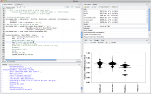
Now, we need to find the right tools to get started with R. After searching a bit, I quickly settled on RStudio. It feels pretty much like a typical IDE with a REPL at its heart. As you can see in the screenshot below, there are four important areas. Top-left are your *.R files in a code editor with syntax highlighting and code completion. Top-right is your current R workspace with all defined variables and functions. This allows also to view and explore your current data set easily. On the bottom-right, we got a window that usually contains either help texts, or plots. Last but not least, in the bottom-left corner is the actual REPL.
Rscript is the interpreter that can be used on the command-line and thus, is nice to have for automating tasks. I installed it using MacPorts.
This introduction is accompanied by a script. It contains all the code discussed here and can be used to follow the introduction avoiding to much copy’n’past. Furthermore, the code here is not as complete as the script, to be a little more concise.
The first thing to do after setting up R is to install some libraries. This can be done easily from the REPL by executing the following code: install.packages("plyr"). This will install the plyr library providing ddply(), which we are going to use later to process our data set. Before it is going to install the code, it will ask for a mirror nearby to download the necessary files. To visualize the benchmark results afterwards, we are going to use bean plots from the beanplot library. The doBy library provides some convenience functions from which we are going to use orderBy(). After the installing all libraries, they can be loaded by executing library(lib_name).
The documentation for functions, libraries, and other topics is always just a question mark away. For instance, to find out how libraries are installed, execute the following code in the REPL: ?install.packages.
Preprocessing Benchmark Results
To give a little context, the experiment this introduction is based on tries to evaluate the impact of using an object table instead of direct references on the performance of our manycore Smalltalk, the RoarVM.
The data set is available here: object-table-data.csv.bz2. Download it together with the script and put it into the same folder. After opening the script in RStudio, you can follow the description here while using the code in RStudio directly. The run-button will execute a line or selection directly in the REPL.
Loading Data
First, change the working directory of R to the directory where you put the data file: setwd("folder/with/data-file.csv.bz2/"). The file is a compressed comma-separated values file that contains benchmark results, but no header line. Furthermore, some of the rows do not contain data for all columns, but this is not relevant here and we can just fill the gabs automatically. Load the compressed data directly into R’s workspace by evaluating the following code:
bench <- read.table("object-table-data.csv.bz2",
                    sep="\t", header=FALSE,
                    col.names=c("Time", "Benchmark", "VirtualMachine",
                                "Platform", "ExtraArguments", "Cores",
                                "Iterations", "None", "Criterion",
                                "Criterion-total"),
                    fill=TRUE)
As you can see in the workspace on the right, the variable bench contains now 60432 observations for 10 variables. Type the following into the REPL to get an idea of what kind of data we are looking at: summary(bench), or View(bench). Just typing bench into the REPL will print the plain content, too. As you will see, every row represents one measurement with a set of properties, like the executed benchmark, its parameters, and the virtual machine used.
Transforming Raw Data
As a first step, we will do some parsing and rearrange the data to be able to work with it more easily. The name of the virtual machine binary encodes a number of properties that we want to be able to access directly. Thus, we split up that information into separate columns.
bench <- ddply(bench,
               ~ VirtualMachine, # this formula groups the data by the value in VirtualMachine
               transform,
               # the second part of the VM name indicates whether it uses the object table
               ObjectTable = strsplit(as.character(VirtualMachine), "-")[[1]][2] == "OT",
               # the third part indicates the format of the object header
               Header = factor(strsplit(as.character(VirtualMachine), "-")[[1]][3]))
This operation could use some more explanation, but most important know now is that we add the two new columns and that the data is being processed grouped by the values in the VirtualMachine column.
The data set contains also results from another experiment and some of the benchmarks include very detailed information. Neither of those information is required at the moment and we can drop the irrelevant data points by using subset.
bench <- subset(bench,
                Header == "full"         # concentrate on the VM with full object headers
                 & Criterion == "total", # use only total values of a measurement
                select=c(Time, Platform, # use only a limited number of columns
                         ObjectTable, Benchmark, ExtraArguments, Cores))
Furthermore, we assume that all variations in measurements come from the same non-deterministic influences. This allows to order the measurements, before correlating them pair-wise. The data is order based on all columns, where Time is used as the first ordering criterion.
bench <- orderBy(~Time + Platform + ObjectTable + Benchmark + ExtraArguments + Cores, bench)
Normalizing Data
In the next step, we can calculate the speed ratio between pairs of measurements. To that end, we group the data based the unrelated variables and divide the measured runtime by the corresponding measurement of the VM that uses an object table. Afterwards we drop the measurements for the VM with an object table, since the speed ratio here is obviously always 1.
norm_bench <- ddply(bench, ~ Platform + Benchmark + ExtraArguments + Cores,
                    transform,
                    SpeedRatio = Time / Time[ObjectTable == TRUE])
norm_bench <- subset(norm_bench, ObjectTable == FALSE, c(SpeedRatio, Platform, Benchmark, ExtraArguments, Cores))
Analyzing the Data
The Basics
Now we are at a point were we can start to make sense of the benchmark results. The summary function provides now a useful overview of the data and we can for instance concentrate on the speed ratio alone. As you might expect, you can also get properties like the standard deviation, arithmetic mean, and the median easily:
summary(norm_bench$SpeedRatio)
sd(norm_bench$SpeedRatio)
mean(norm_bench$SpeedRatio)
median(norm_bench$SpeedRatio)
However, that is very simple, a bit more interesting are R’s features to query and process the data. The first question we are interested in is, whether there is actually an impact on the performance difference for different numbers of cores:
summary(norm_bench$SpeedRatio[norm_bench$Cores==1])
summary(norm_bench$SpeedRatio[norm_bench$Cores==16])
Beanplots
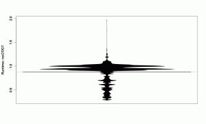
Starring at numbers is sometimes informative, but usually only useful for small data sets. Since we humans are better in recognizing patterns in visual representations, beanplots are a better way to make sense of the data. They are an elegant visualization of the distribution of measurements.
beanplot(SpeedRatio ~ Platform,
         data = norm_bench,
         what = c(1,1,1,0), log="",
         ylab="Runtime: noOT/OT",
         las=2)
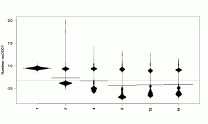
This beanplot tells us, like the numbers before, that the mean is smaller than 1, which is the expected result and means that the indirection of an object table slows the VM down. However, the numbers did not tell use that there are various clusters of measurements that now become visible in the beanplot and are worth investigating.
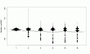
Let’s look at the results split up by number of cores.
beanplot(SpeedRatio ~ Cores,
         data = norm_bench,
         what = c(1,1,1,0), log="",
         ylab="Runtime: noOT/OT")
Digging Deeper
While noticing that the variant without object table is faster for more cores, we also see that the speed ratios are distributed unevenly. While the bean for 1-core has a 2-parted shape, the 2-cores bean has a lot more points where measurements clump. That is probably related to the benchmarks:
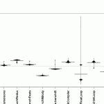
beanplot(SpeedRatio ~ Benchmark,
         data = subset(norm_bench, Cores==2),
         what = c(1,1,1,0), log="",
         ylab="Runtime: noOT/OT", las=2)
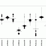
beanplot(SpeedRatio ~ Benchmark,
         data = subset(norm_bench, Cores==16),
         what = c(1,1,1,0), log="",
         ylab="Runtime: noOT/OT", las=2)
Those two graphs are somehow similar, but you might notice that the float loop benchmark has a couple of strong outliers. I forgot the exact identifier of the float loop benchmark, so lets find out with this code: levels(norm_bench$Benchmark)
Now let’s filer the data shown by that benchmark.
beanplot(SpeedRatio ~ Cores,
         data = subset(norm_bench, Benchmark == "SMarkLoops.benchFloatLoop"),
         what = c(1,1,1,0), log="", ylab="Runtime: noOT/OT")
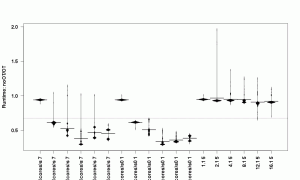
This visualization reassures me, that there is something strange going on. The distribution of result still looks clumped as if there is another parameter influencing the result, which we have not regarded yet. The only column we have not looked at is ExtraArguments, so we will add them. Note that droplevels() is applied on the data set this time before giving it to the beanplot() function. This is necessary since the plot would contain all unused factor levels instead, which would reduce readability considerably.
beanplot(SpeedRatio ~ Cores + ExtraArguments,
         data = droplevels(subset(norm_bench, Benchmark == "SMarkLoops.benchFloatLoop")),
         what = c(1,1,1,0), log="", ylab="Runtime: noOT/OT", las=2)
Fixing up a Mistake
This plot now shows us that there are three groups of results with different ExtraArguments. Think I forgot that the data set contains some very specific benchmarks. The overall goal of the benchmarks is to test the weak scaling behavior of the VM by increasing work-load and number-of-cores together. However, for the questions we are interested here, only those weak-scaling benchmarks are of interest. Thus, we need to filter out a couple of more data points, since the results will be unnecessarily biased otherwise. To filter the data points we use grepl. It matches the strings of ExtraArguments and allows us to filter out the single-core and the 10x-load benchmarks.
norm_bench <- subset(norm_bench,
                     !grepl("^1 ", ExtraArguments)    # those beginning with "1" put load on a single core
                     & !grepl("s0 ", ExtraArguments)) # those having "s0" in it put 10x load on each core
norm_bench <- droplevels(norm_bench)
And since I always wanted to say that: The exercise to regenerate all interesting graphs and re-answer the original questions are left to the interested reader. 😉
Conclusion
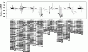
As a final graph, we can plot all benchmarks for all cores, and get an overview. The par function allows to adapt the margins of the plot, which is necessary here to get the full benchmark names on the plot.
par(mar=c(20, 4, 1, 1))
beanplot(SpeedRatio ~ Cores + Benchmark,
         data = norm_bench,
         what = c(1,1,1,0), log="",  ylab="Runtime: noOT/OT", las=2)
As we already knew, we see an influence of the number of cores on the results, but more importantly, we see most benchmarks benefitting from removing the extra indirection through the object table. The float loops benefit by far the strongest. The float objects are so small and usually used only temporary that avoiding the object table pays off. For the integer loops it does not make a difference, since the VMs uses immediate values (tagged integers). Thus, the integers used here are not objects allocated in the heap and the object table is not used either.
Beyond the won insight into the performance implications of an object table this analysis also demonstrates the benefits of using a language like R. Its language features allow us to filter and reshape data easily. Furthermore, regenerating plots and tracing steps becomes easy, too. Here it was necessary since some data points needed to be removed from the data set to get to reasonable results. Reexecuting part of the script or just exploring the data is convenient and done fast, which allows me to ask more questions about the data and understand the measurements more deeply. Furthermore, it is less a hassle to reassess the data in case certain assumptions have changed, we made a mistake, or the data set changed for other reasons. From my experience, it is much more convenient than Excel, but that might just be because I spend more time on learning R than on learning Excel.
In case you try it out yourself, you will certainly want to experiment with other types of visualizations, save them to files, etc. A few of these things can be found in my benchmarking scripts on GitHub: BenchR.
 I head the
